This week I put two new preprint on the arXiv. Both are on a similar theme, so I will discuss them together. One is with Morgan Rodgers on regular sets of lines in rank 3 polar spaces. The other one is solves a problem which I have been thinking about very regularly since November 2017: The classification of Boolean degree  functions (or Cameron-Liebler classes) of
  -spaces in an
  -dimensional vector space
  over the field with
  elements for large enough (and and
  fixed).
Not only did I (and many other researcher) try to solve this problem for many years, it also turns out that the solution has a very short and concise proof. So for now I am very happy about it. [And please do not find a mistake. Any mistake must be embarrissingly simple.] The problem itself (for  ) goes back to a paper by Cameron and Liebler in 1982, so it is also a reasonably old problem.
1. Definitions
One beautiful thing about Cameron-Liebler sets is that one can think about them in various ways (see my old post here for definitions): as Boolean homogeneous degree polynomials on vector spaces, as families of -spaces which have on average large intersections with each other, as extremal regular sets or equitable bipartitions, as the sets in the the span on maximal intersecting families (what finite geometers call textit{point-pencils}), or as sets which intersect each spreads (partitions of into -spaces) in the same number.
For here one definition suffices:
Put weights on the -spaces of , say, using some map  from the -spaces of to the real numbers. If we can do so such that all -spaces have either weight
  or (where the weight of a -space is simply the sum of the weights of its -spaces), then we have a Boolean degree function or Cameron-Liebler class.
[I like this definition because (for me) it makes all the other equivalent definitions clear. Say, if I want to understand why a Boolean degree polynomial is the same as a set which intersects each partition of into -spaces in a constant number, then my thought process passes through .]
There are the trivial examples:
- Example (I). Put the weight on everything. Then each -space has weight .
- Example (II). Put the weight on one -space
 and the weight on everything else. Then each -space through has weight , all others have weight .
- Example (III). Put the weight
 on all -spaces in a hyperplane
  and weight
  on all the other -spaces. Then the -spaces in have weight , all others have weight .
- Example (IV). The same as before, but put change the weight of one -space not in , such that all -spaces through also have weight .
- The complement of any of the previous examples.
Are there any other examples? Yes, many are known for  and . I list references to the most important ones in my preprint. For
  , we know that no other examples exist as soon as
  . Many people (starting with Cameron and Liebler in the 1980s, and Keldon Drudge, whose PhD thesis we will discuss below, in the 1990s) seemed to believe that there are no other examples for large enough compared . Yuval Filmus and I formally stated this as a conjecture in our joint paper in 2018 on the topic. Now let’s discuss the three elements of the proof which proves this conjecture.
2. The Proof: Ramsey (Graham, Leeb, Rothschild), Drudge, and Metsch
First let us list the ingredients for the proof. In general, we will identify the set  of -spaces of weight with the Boolean degree function (or Cameron-Liebler set).
Ingredient 1: It is enough to show the claim for for some fixed and . That was shown by Yuval Filmus and me in 2018. That fixed is easy to see. Probably, already Cameron and Liebler knew that, but Drudge wrote it very conretely in his PhD thesis in 1998. I think of -spaces as projective points and of  -spaces as projective lines.
Ingredient 2: If we limit ourselves to a  -space and the set of lines of in that -space corresponds corresponds to Example (II) or Example (III), then the example in the whole space corresponds to Example (II) or Example (III). This was shown by Drudge in his PhD thesis in 1998. The main thing here is that we only need to find Example (II) or Example (III) in some subspace of our larger vector spaces.
Ingredient 3: If we only have weights which occur in one of the examples (I)–(V), then one necessarily has one of the examples (I)–(V). This is true for numerical reasons and for the fact that the examples (I)–(V) must be very different in size from all other examples. There are several stability results for Cameron-Liebler line classes which show this, many involving Klaus Metsch. For my purposes his result from 2010. It states for and that if  , then either
  and is one of examples (I)–(V), or
  .
.
Ingredient 4: For fixed , only a finite list of weights can occurs. That is because for  and , we have a projective plane and the point-line incidence matrix of a projective plane has full rank. A projective plane over a field with elements has
  lines, so we have at most
  non-isomorphic sets of lines. For each set of lines, each point will get a weight. Hence, we have at most
  weights occurring.
Ingredient 5: We all know Ramsey’s theorem. It states that if for some fixed we color the elements of a set  of size with
  colors, then for all sufficiently large there exists a -set
  in such that all elements of have the same color. In an old and celebrated result, Graham, Leeb, and Rothschild generalized this to affine and projective spaces, that is we color -spaces and find a monochromatic -space for large enough (with
  fixed).
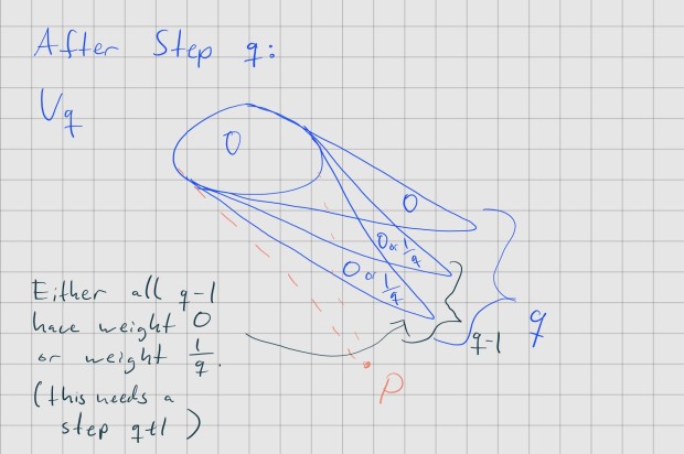
So how does the proof go? We use Ingredient 5 (with the from Ingredient 4) several times to pull out subspaces with constant weight. Subspaces of constant weight will have one of the weights occurring in the examples (I)–(V), so this is already good. But one needs to do this in a slightly clever way because we want to use Ingredient 3. One does this iteratively by taking one point whose weight one wants to figure out. Then one looks at smaller and smaller subspaces 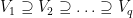 of such that always stays in these
  , but also such that we collect parallel affine hyperplanes of uniform weight in these . Then we need to pick some
  without to say something about the uniform weights which can occur, go back to , and then see that must have one of the weights in examples (I)–(V). Using Ingredient 3, we are done.
Below you can find a visualization of the construction which I find helpful. I sincerely apologize for my handwriting.
I like this argument as it is very simple. Also, applications of Ramsey results to finite geometry seem to occur mostly to made-up problems. Here we have a decades old question for which a Ramsey result could be utilized.
Note that I mention the PhD thesis by Bernd Voigt from 1978 in my preprint. Thanks to Lukas Kühne (who scanned it for me) and Hans Jürgen Prömel (who told me about it) I could read it. In there Bernd Voigt shows a nice generalized version of the Ramsey result by Graham, Leeb and Rothschild which I found very readable. If I find the time, I will put an English translation on the arXiv in the next few weeks as I like its generality. A German version of a special case was published in the European Journal of Combinatorics. There is also a short proof due to Spencer which I find easier to read than the proof by Graham, Leeb, and Rothschild. All of these results are applications of the Hales-Jewett theorem.
Can we classify Boolean degree functions close to degree ? This would be a Friedgut-Kalai-Naor (FKN) theorem for vector spaces. My argument for the classification uses some specific results, but much of it appears to be generic as long as there is a suitable Ramsey result available. What is the right larger class of problem to solve with this method? Can we classify degree function?
3. Regular Sets in Finite Geometry
My other preprint this week was with Morgan Rodgers. It is on regular sets of graphs. The Cameron-Liebler sets discussed in the above are regular sets. Say, you have a regular graph  with adjacency matrix
  , then will have some eigenspaces
  ,
,  , …,
, …,  , where usually
  is the span of the all-ones vector. Having a regular set or equitable bipartition (as discussed here) is equivalent to having a set of vertices such that the characteristic vector of that set is in
  for some
  .
.
If is the Grassmann graph, that is the graph with the -spaces of an -dimensional vector space as vertices, two adjacent if they meet in a  -space, then we are in the setting of Cameron-Liebler sets as discussed above. There we asked for a classification of regular sets in
  and we succeeded in classifying them.
With Morgan I investigated regular sets in graphs related to polar spaces. There has been much work done on regular sets on the point graphs of polar spaces (these are called  -ovoids and
  -tight sets), and on maximal totally isotropic subspaces of polar spaces. This is because here the corresponding graphs are particularly nice and are strongly regular for points and distance-regular for maximal isotropic subspaces. Due to some other work which Morgan was doing with Maarten De Boeck and Jozefien D’haeseleer, he got interested in the graph of lines in polar spaces of rank
  .
.
Say, you have a rank polar space. Then you have totally isotropic -spaces (points), -spaces (lines), and -spaces (planes). Two lines can be in the following relations:
- They are identical.
- They meet in a point and are contained in plane.
- They meet in a point, but are not contained in a plane.
- They are disjoint, but there exists a plane which contains one of the lines and meets the other line in point.
- They are disjoint, but not the previous case. This is oppositeness in a building theoretic sense if you like building theory, also see my first proper blog post.
Each of these relations can define a graph and one can ask for a classification (or structural result) about the regular sets in this setting. Originally, I was not sure how interesting this project will. A posteriori it turns out that many interesting structures from finite geometry appear:
This makes me think that such regular sets of lines are interesting in general. And it even gave a new construction for the problem in the work by Jozefien, Maarten, and Morgan! See the preprint for details.